
Welcome back to our Impacter plug-in blog series. In the previous two blogs we mostly covered the physical parameter aspects of the plug-in and how they can integrate well with your game’s physics system. In this blog we discuss the other aspect of Impacter: its capacity for cross synthesis.
As we saw briefly in the first Impacter blog, the possibility of mixing and matching the “impact” and “body” components of different sounds can be used to create novel variations within a group of sounds. We even implemented a random playback behaviour in the plug-in to allow designers to easily make use of these variations.
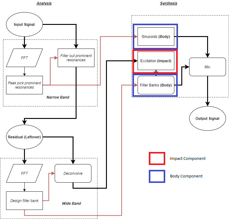
Recall that cross synthesis variations are produced by taking the “Body” (Sinusoids & Filter Banks) and “Impact” (Excitation) components in the synthesis module from different sounds.
Cross synthesis, however, is a very broad term and it is useful to go into more detail about what kind of variations one might expect from Impacter’s particular flavour of cross synthesis. We would like to be able to demonstrate that the variations users can produce with Impacter are real and coherent; that variations are not redundant, but still related to the original sounds in a meaningful way. We’d also like to be able to assure designers that the player should not encounter repetitions of sounds that would break the immersion in gameplay, either by being too repetitive or by being too unrelated. As we will see, providing such a useful description of Impacter’s cross synthesis is not as easy as it may seem.
Looking at Variations, Listening to Variations
Impacter allows every file loaded into the plug-in to be cross synthesized with every other loaded sound. 12 files, for example, allows for up to 144 combinations (the user can omit certain impact and body components in the source editor). What becomes immediately obvious is that 144 impact sounds becomes too many to listen to, or even look at, in order to discern any meaningful difference between sounds.
For example:
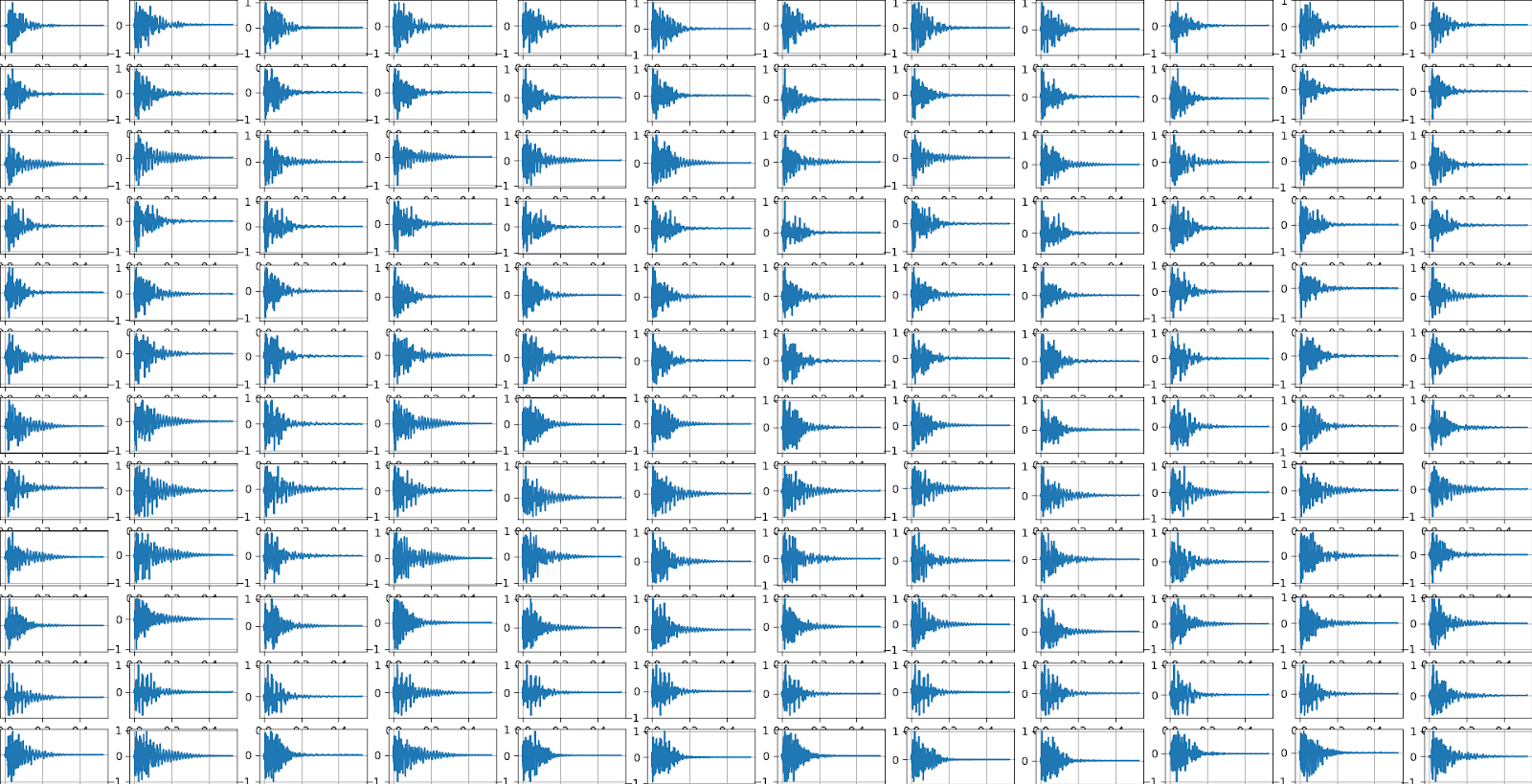
And for sake of saying, it would clearly be unreasonable to listen to these in order and remember what sound #11 sounded like once you get to sound #87..
So what can we do to parse this overwhelming amount of sounds?
Dimensionality Reduction
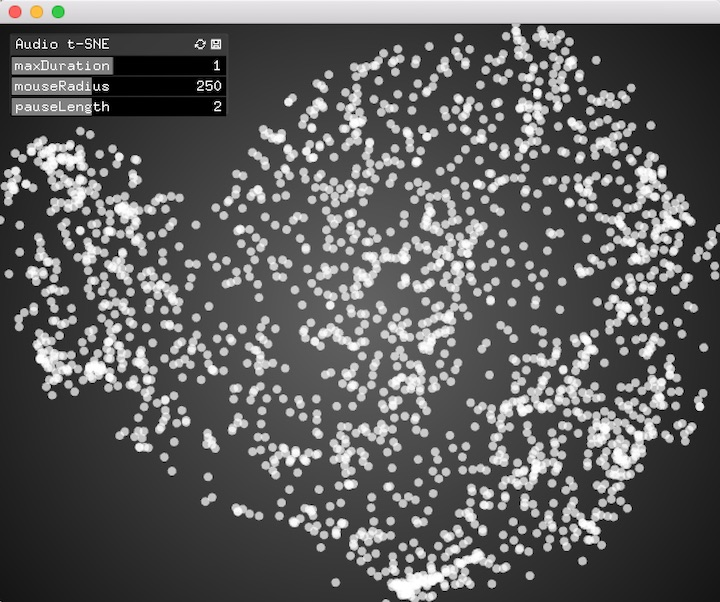
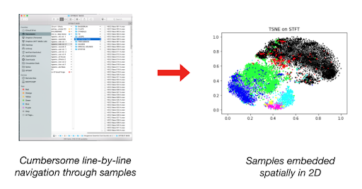
As a technique for audio analysis more broadly, dimensionality reduction allows us to map a large collection of sounds onto a 2D plane to look at. Lamtharn “Hanoi” Hantrakul’s Klustr blog and accompanying tool [1], as well as the ml4a (Machine Learning for Artists toolkit) “Audio t-SNE” viewer [2] are both excellent examples of what dimensionality reduction for audio looks like.
Comparing Latent Features of Impact sounds
There are many ways to “compare” sounds in 2D space. Impact sounds have an intuitive set of latent features: their physical characteristics (hard, soft, bounce, strike), or the type of object or surface being impacted (glass, sand, wood). We can’t explicitly define (in mathematical terms) what the latent features of a sound are that we are looking for, but we can try to extract various audio features from a sound to compare.
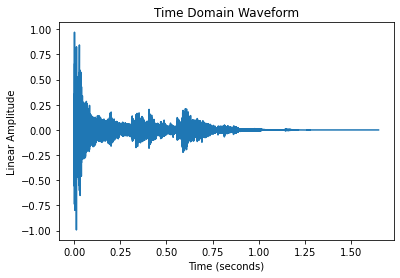
When working with audio, comparing the raw time domain signal above is often not ideal for comparing different sounds. There is fortunately a wide world of audio analysis techniques to transform each sound into a more comparable form. As we’ll see later, the choice of audio analysis directly affects the resulting plots produced by dimensionality reduction.
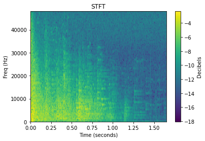
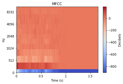
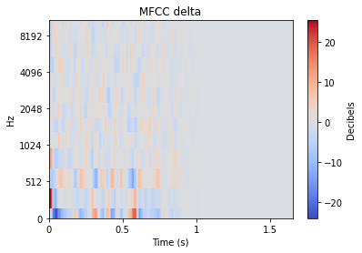
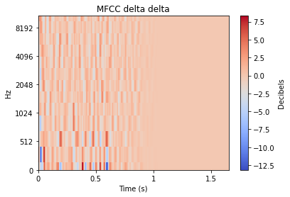
There is plenty of reading that one can delve into about each of these transformations, but for the sake of this article we’ll simply provide a visual example of the transformation applied to an impact type sound. Many of these transformations often expand a 1D audio signal into 2D, and so the level of each value is represented by colour.
AUDIO FEATURES |
|
 |
 |
 |
 |
Since dimensionality reduction is ultimately providing a visual comparison of sounds, we can think intuitively about how we might expect the STFT of two sounds to differ, versus how the MFCCs might differ. It is not as expressive as comparing, say, the latent aspects of sounds: “drum” sounds versus “trombone” versus “gravel” sounds. However, audio features might still end up creating a 2D map that approximates the latent differences between sounds well enough.
What Dimensionality Reduction Does
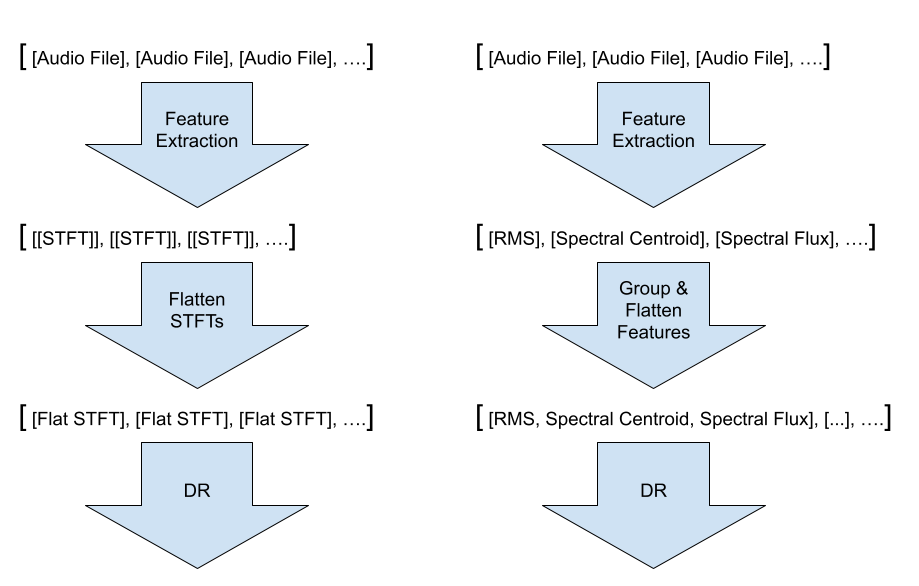
Now that we have audio features, dimensionality reduction can “reduce” the list of numbers associated with each sound in a collection (as in the figure below) to a collection of 2 number lists, or pairs, which conveniently map onto the X-Y coordinates of a two dimensional plane. Importantly, however, we want the proximity or distance between sounds in the 2D plane to be reflective of meaningful similarities or differences in the sound. In a sense, it is a way of simplifying the visual comparison between all the sounds (or features) we’ve looked at above.
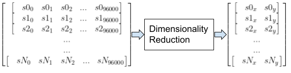
A collection of sounds each 2 seconds long at 48k sample rate, which would each be 96000 samples long, being reduced to a collection of 2D coordinates
In summary, the whole “dimensionality reduction” pipeline looks something like this:
| SOUND | FEATURE EXTRACTION | DIMENSIONALITY REDUCTION | 2D PLOT |
|
|
|
 |
Visualizing Impacter Cross Synthesis
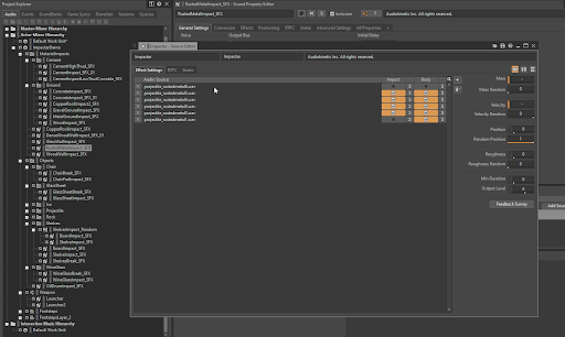
To get a good result from dimensionality reduction, you need to work with a large enough group of sounds. Fortunately for us, we have on hand a live Wwise project with plenty of Impacter variations to analyze: The Impacter Unreal Demo! (Read the blog here!)
The Impacter demo project has 289 sounds over multiple Impacter instances, which culminates in a total of 2295 possible variations to examine. For our experiments, we were able to run an offline version of our Impacter algorithm to generate all these variations, and then compare the results of trying various audio feature extraction methods as inputs, and various dimensionality reduction algorithms to generate plots.
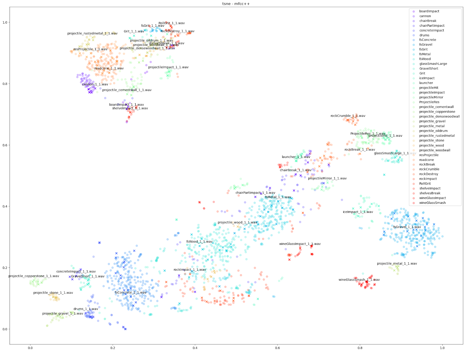
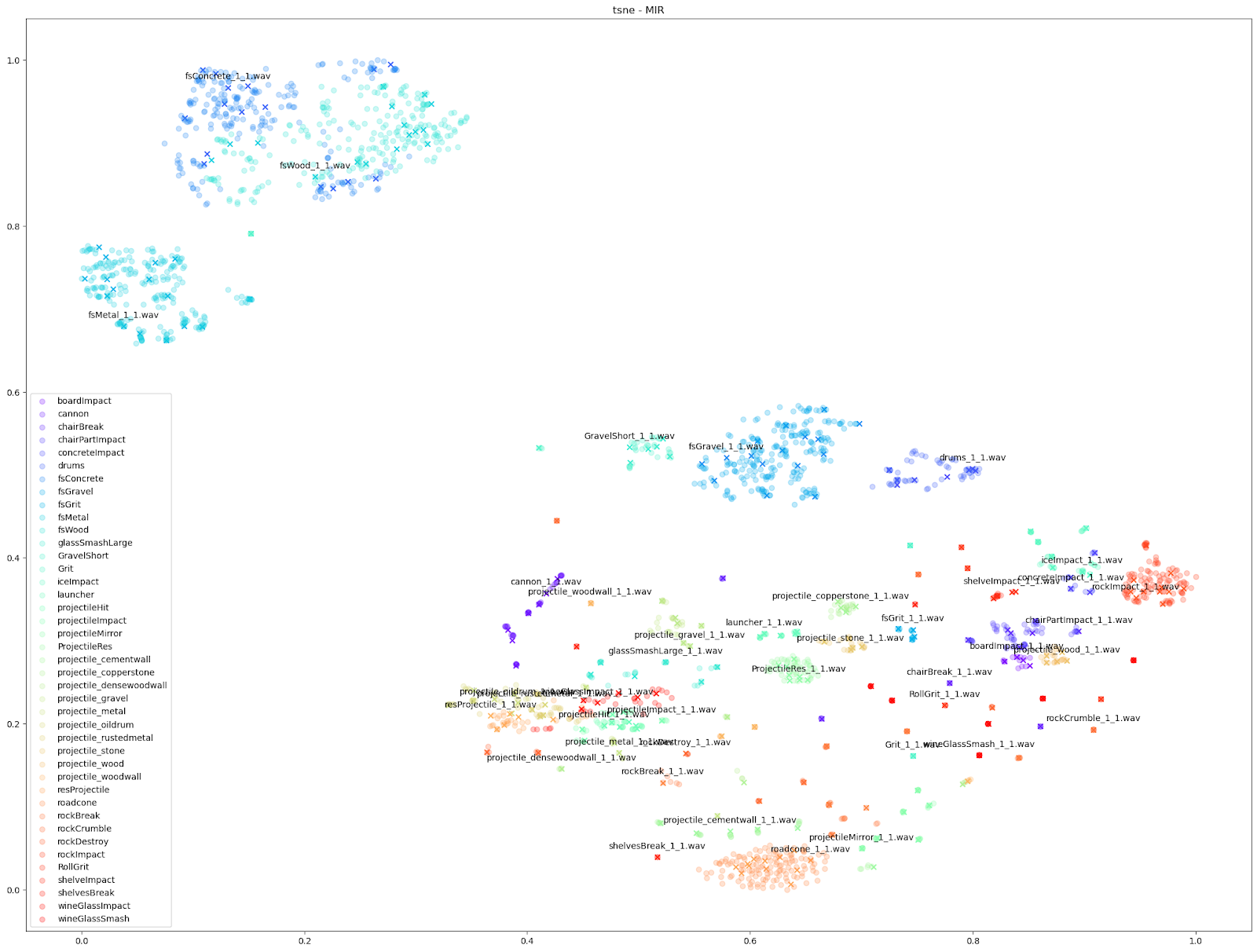
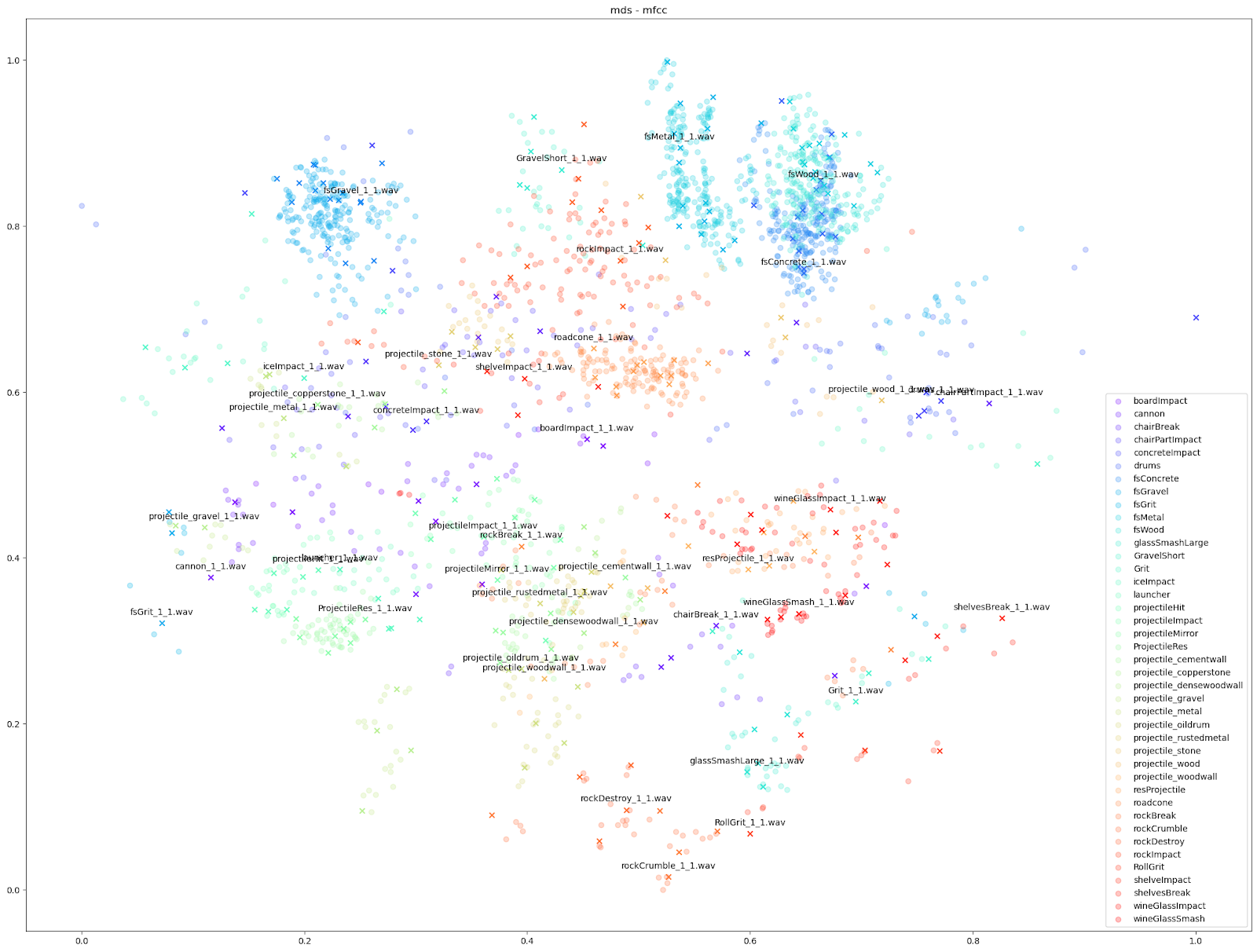
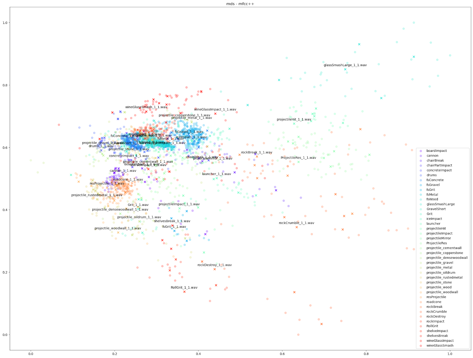
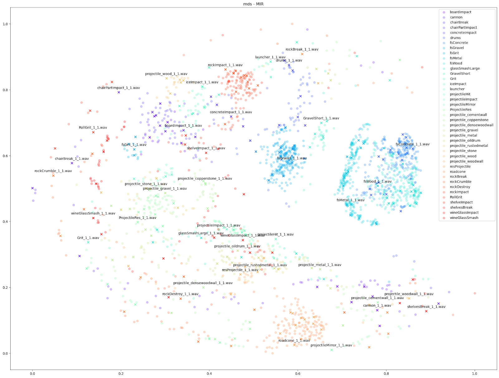
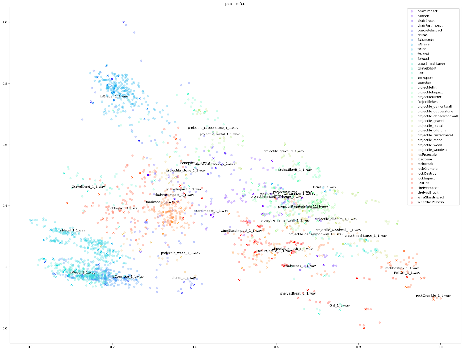
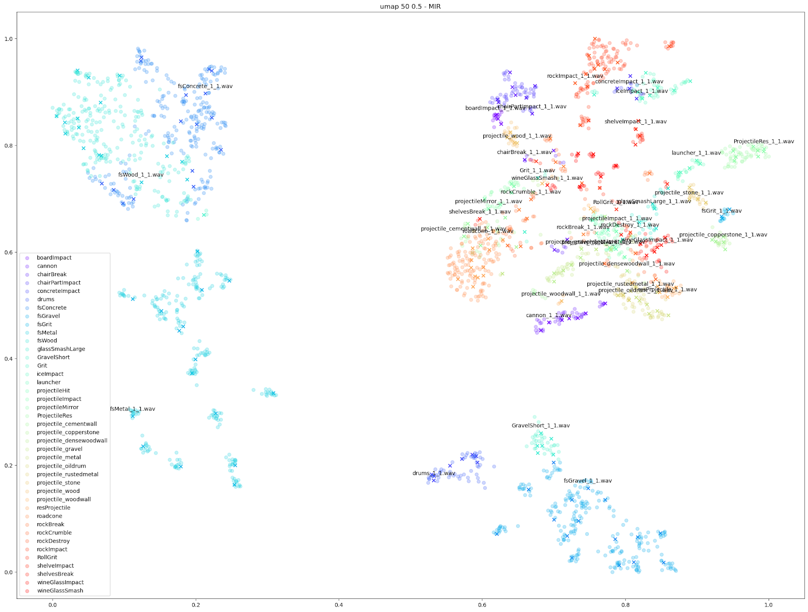
Since we know which sounds come from which Impacter instance, we are able to assign a colour to each Impacter SFX, and different shapes to distinguish the original sounds from the variations. In the cases below, we use an ‘X’ to denote the original input sounds, and a circle for the variations produced by Impacter. The colour coding can help show how coherent the variations are: they will be in close proximity to their original of the same colour, and also show that the variations are not redundant: they will not be on top of one another.
We tried a few different audio features and dimensionality reduction algorithms, and included the broader results at the bottom of this blog, but here are our favourite results:
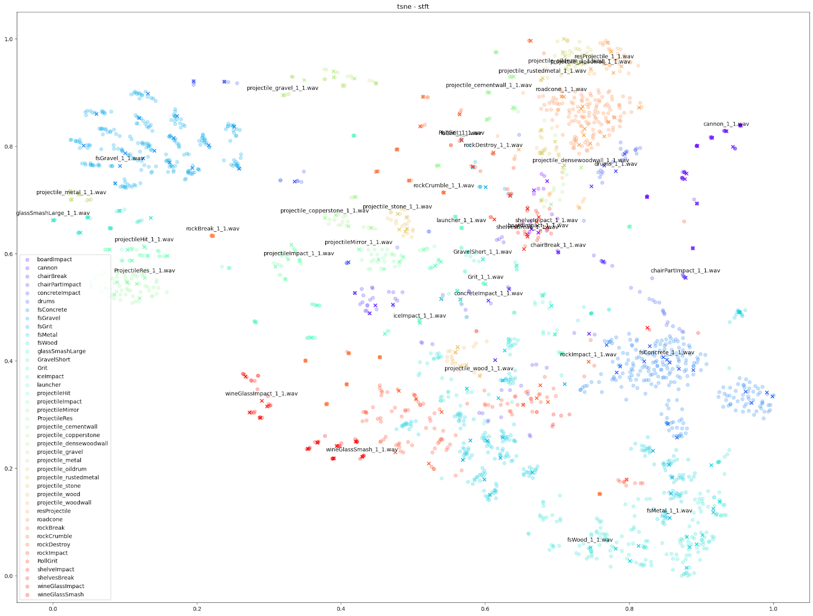
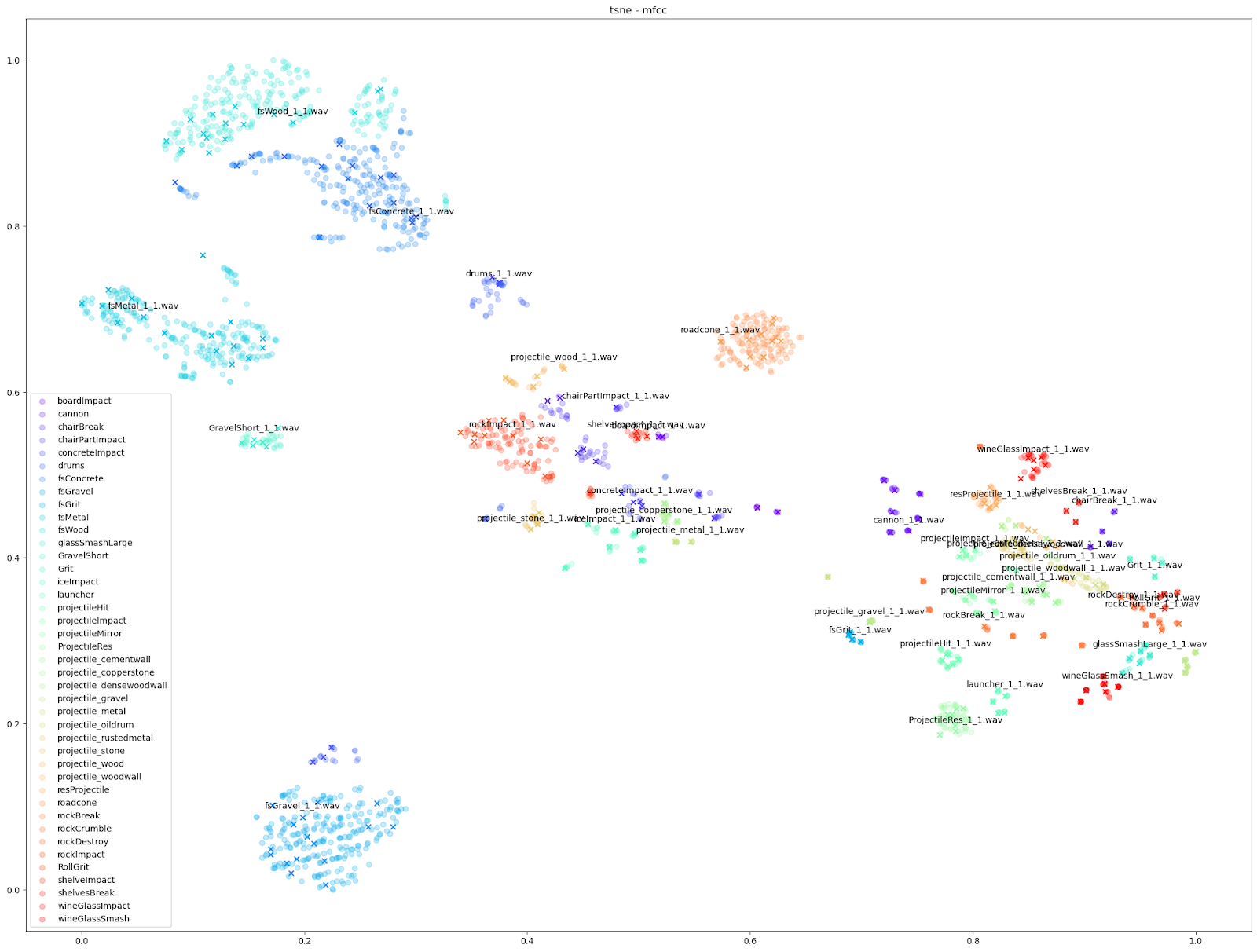
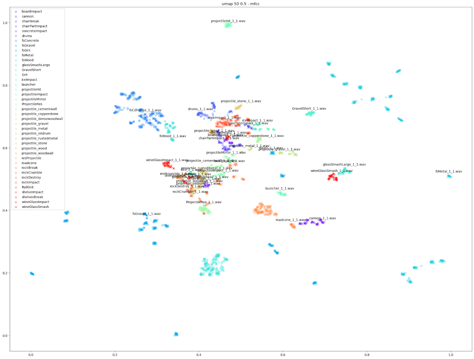
We can see in all cases that there is at least some balance of differences between originals and variations with each Impacter instance (by colour). Impacter is not not just generating randomness either: the colour coded sounds still end up clustered near one another, demonstrating a coherence between variations and their originals.
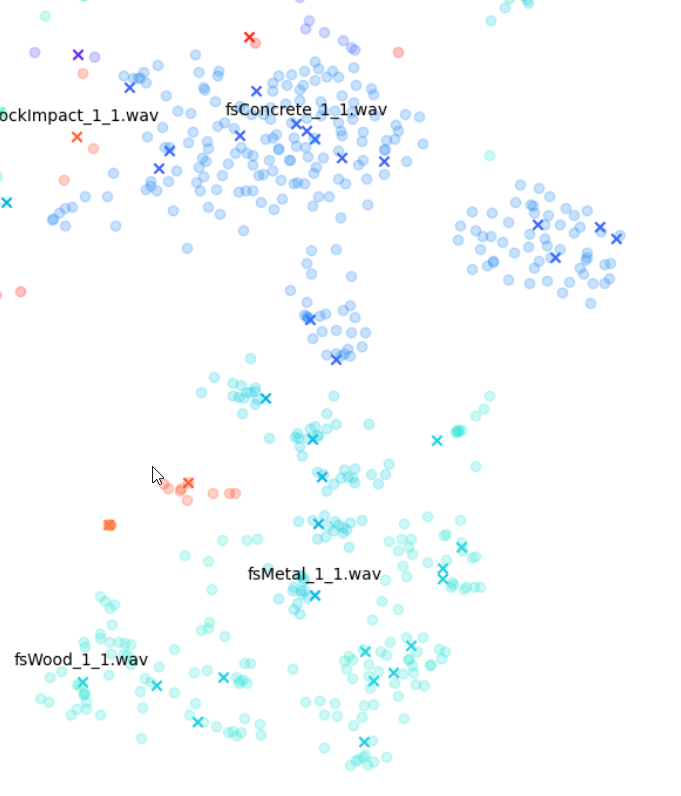
Examining the plot of t-SNE on STFT features up close, we can see the kind of mixed extent of variation amongst the STFTs of each Impacter sound. The ideal cases in the bottom right - the concrete, wood and metal sounds - show an almost uniform displacement of sound variations around the originals.
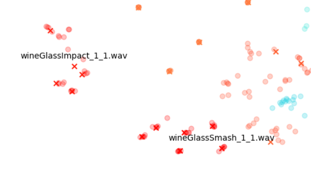
On the other hand, the wineglass or cannon sounds with the dots almost stacked on top of the X’s, show that the STFTs of each variation are much more similar to their originals.
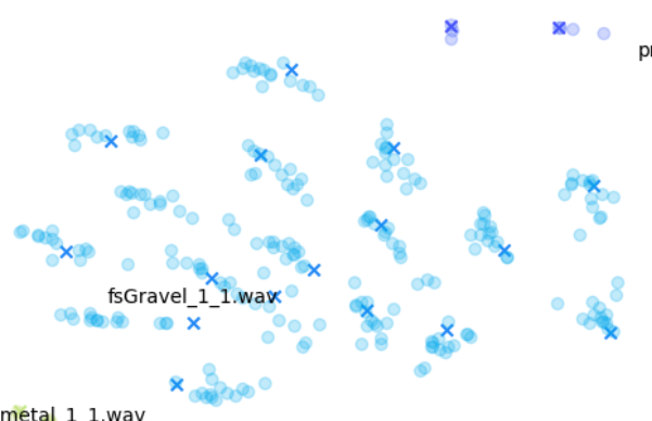
The gravel in the top left, comparatively, is a kind of middle ground where there are obvious variations, but the variations around each original file are disparate from other variation-original file clusters.
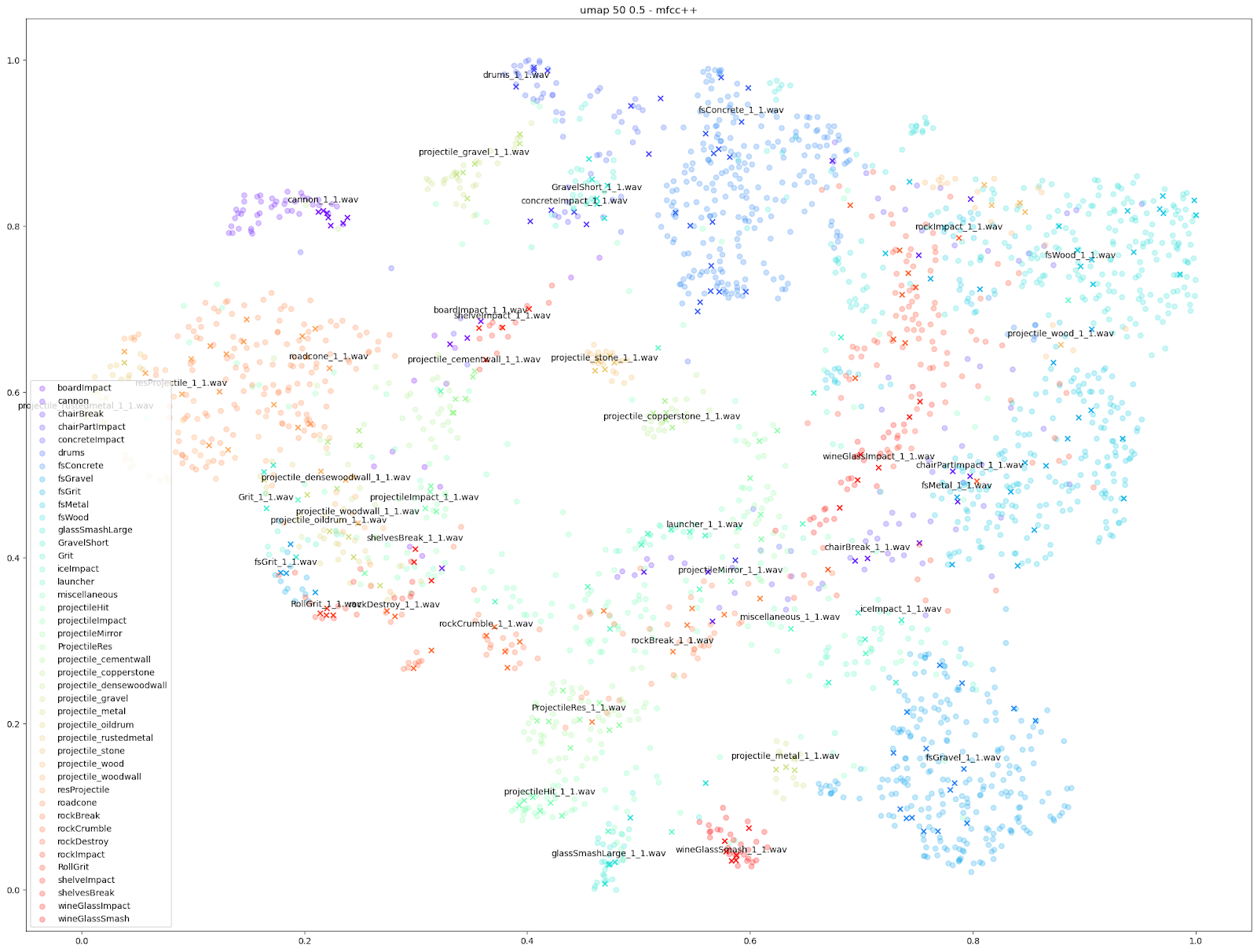
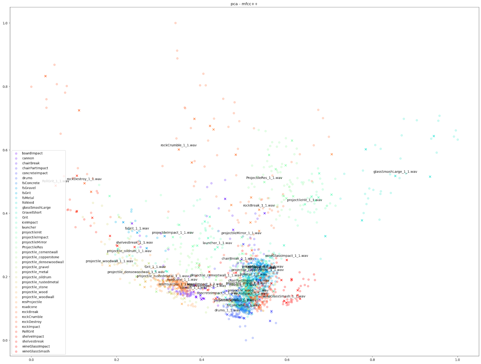
Other audio features can emphasize smaller differences however, such as the “mfcc++” plots. The inclusion of the first and second deltas (the '++' part of 'mfcc++') [3] increases the spread among clusters that would be more bunched together under the STFT plot, such as the wine glass clusters.
.png)
Now we have a plot that expands the differences between sounds in 2D space in such a way that it allows us to see all the variations at once, and even zoom in on particular sounds to see how they vary locally. It looks cool, but it also provides a useful anecdote about how Impacter works.
Impacter is an analysis and synthesis system that models impact sounds, and different input sounds can be better or worse modeled by the algorithms. With these plots, we can informally gauge how well a sound is modeled by Impacter. As we can see, glass sounds only vary so much, and thus we might say are not as ideally modeled by Impacter as the metal, wood and concrete sounds are. This may seem obvious, but it’s an important heuristic to keep in mind when choosing sounds for Impacter - the efficacy of the cross synthesis features will depend on the sound. In short: some sounds will vary more, others less!
None of this is a formal proof of Impacter’s correctness of course, but rather a kind of anecdote to convey all the differences between a large collection of sounds in an intuitive way, and an excuse to experiment with some exciting data visualization techniques along the way.
Other questions
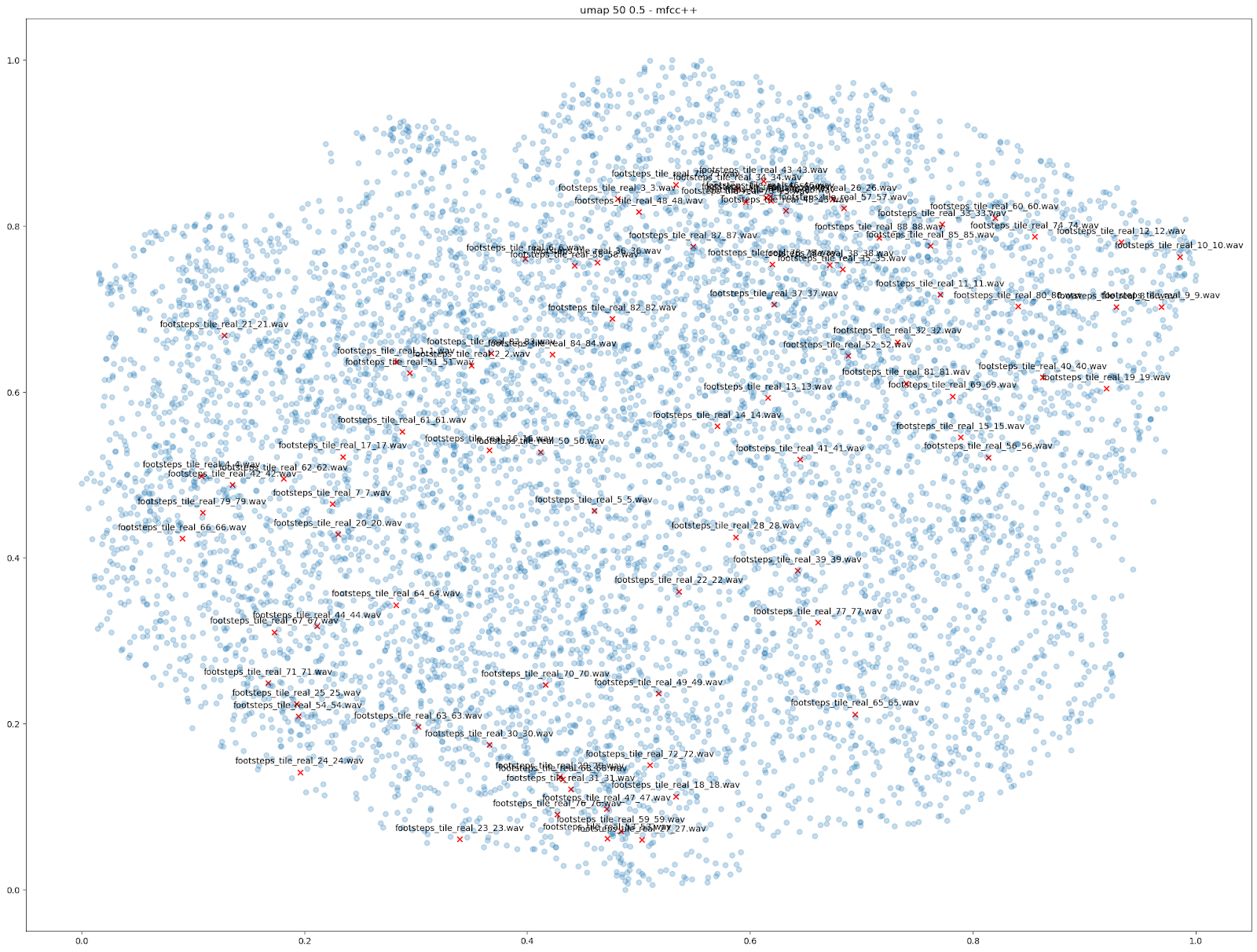
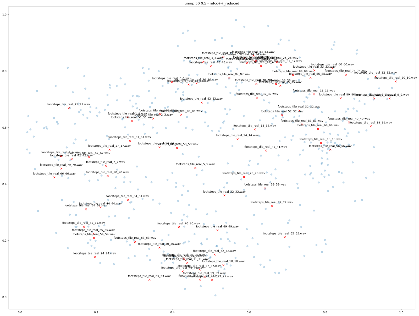
There are other comparisons we can make using dimensionality reduction to visualize what Impacter can do. One thing we tried was visualizing the variations produced among 88 different footstep sounds on tile, leading to a total of 7744 tile sounds. Again, examining the ‘MFCC++’ features plotted by UMAP demonstrates the usefulness of Impacter: variations occur in between the original sounds. What this shows is that some smaller set of those 88 sounds put into Impacter could reconstruct a similar range of variation that the original 88 sounds covered. The second image shows the variations produced by only 22 of the original sounds, along with all 88 originals.
| VARIATIONS FROM 88 FOOTSTEPS | VARIATIONS FROM A SUBSET OF 22 FOOTSTEPS |
 |
|
Right click image "Open in new tab" for larger view.
Conclusion
Hopefully this blog helps answer the question of what kind of variations the Impacter cross synthesis algorithm produces. As we’ve said above, it’s by no means an exhaustive or statistical proof that all variations are exactly different, but hopefully an intuitive way of looking at the large collections of sounds that the plug-in might produce, to give you a better idea of what you’re working with when you use Impacter.
Further Details…
A note on data formatting
Dimensionality reduction algorithms simply accept a collection of data lists, or vectors. Since the dimensionality reduction algorithm is agnostic to the input data, and doesn’t account for the dimensions in 2D input data like STFTs or MFCCs, we can actually flatten 2D data, and even concatenate multiple features from above into a single list to provide to the algorithm.
Dimensionality Reduction Algorithms
There are many existing dimensionality reduction algorithms which simply accept a collection of data lists, or vectors, which in our case are each sound’s features we extracted in the first step.
The sklearn and umap-learn packages in Python (available on pip) provide implementations of many useful dimensionality reduction algorithms that we’ll use. Again, a great deal has been written about how these algorithms work, but for the sake of this article we’ll simply provide links for further reading.
t-distributed Stochastic Neighbor Embedding (t-SNE)
from sklearn.manifold import TSNE
tsne = TSNE(
n_components=tsne_dimensions,
learning_rate=200,
perplexity=tsne_perplexity,
verbose=2,
angle=0.1).fit_transform(data)
Uniform Manifold Approximation and Projection for Dimension Reduction (UMAP)
import umapumap = umap.UMAP(
n_neighbors=50,min_dist=0.5,n_components=tsne_dimensions,metric='correlation').fit_transform(data)
Principal Component Analysis (PCA)
from sklearn.decomposition import PCApca= PCA(n_components=tsne_dimensions).fit_transform(data)
Multidimensional Scaling (MDS)
from sklearn.manifold import MDSmds = MDS(
n_components=tsne_dimensions,verbose=2,max_iter=10000).fit_transform(data)
All Results
For our test on Impacter, we compared the four dimensionality reduction algorithms from above. We ran each algorithm with various sets of audio features as inputs: the STFT and MFCC, the MFCC with it’s delta and delta-delta appended (mfcc++) [3], and finally a concatenation of a variety of audio features (rms, spectral centroid, spectral crest, spectral flux, spectral rolloff, zero crossing rate).
| STFT | mfcc | mfcc++ | “Audio Features List” | |
| t-SNE |  |
 |
 |
 |
| MDS | 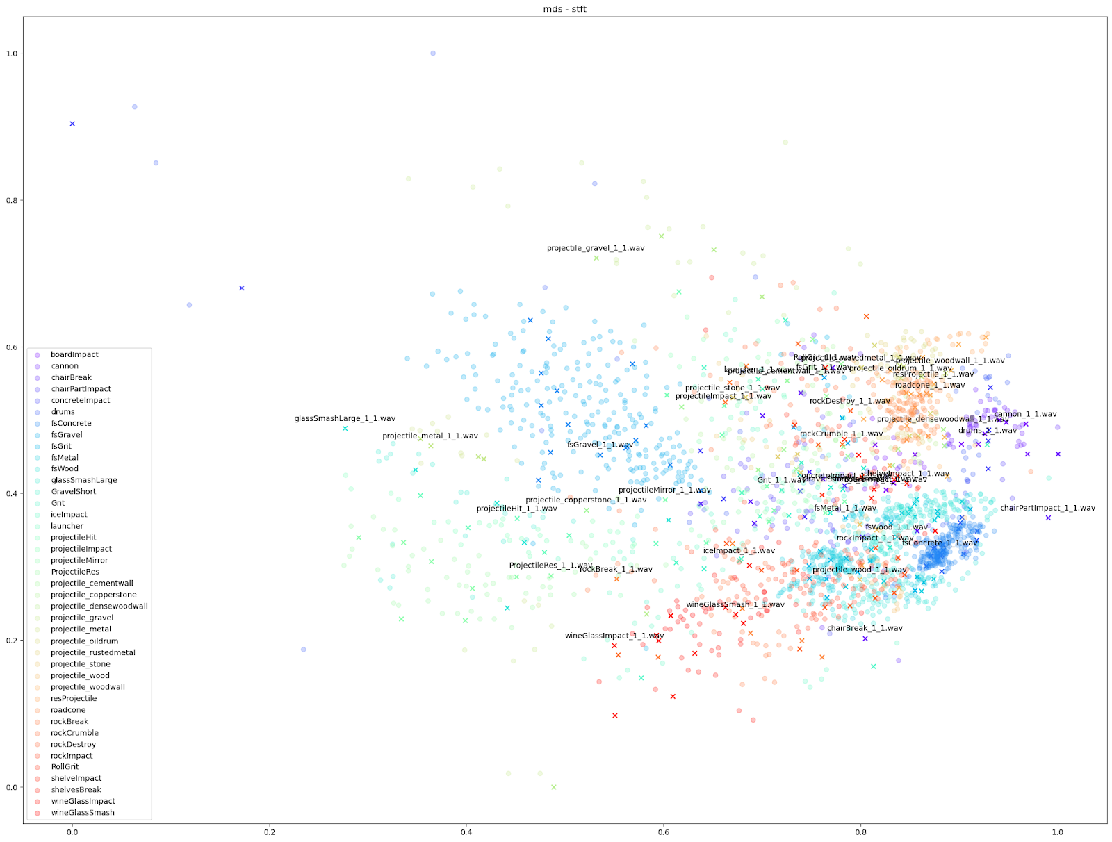 |
 |
 |
 |
| PCA | 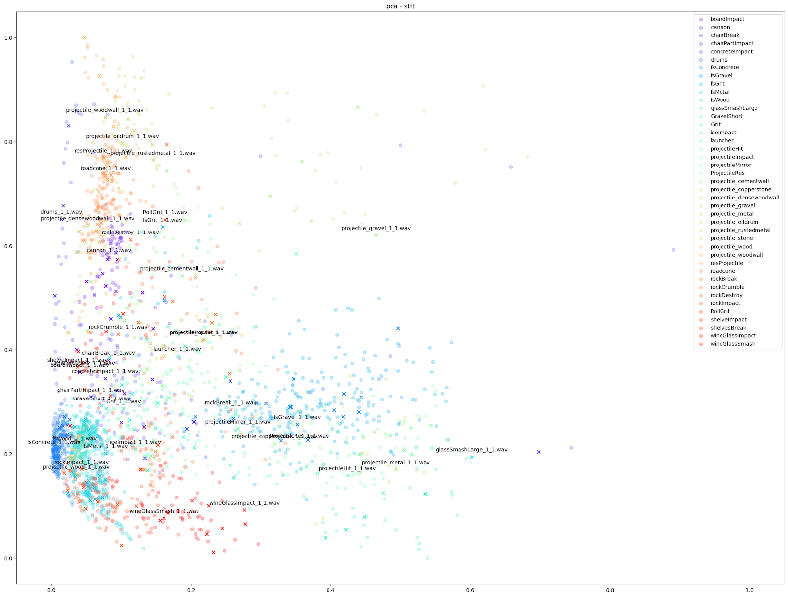 |
 |
 |
 |
| UMAP 50 0.5 | 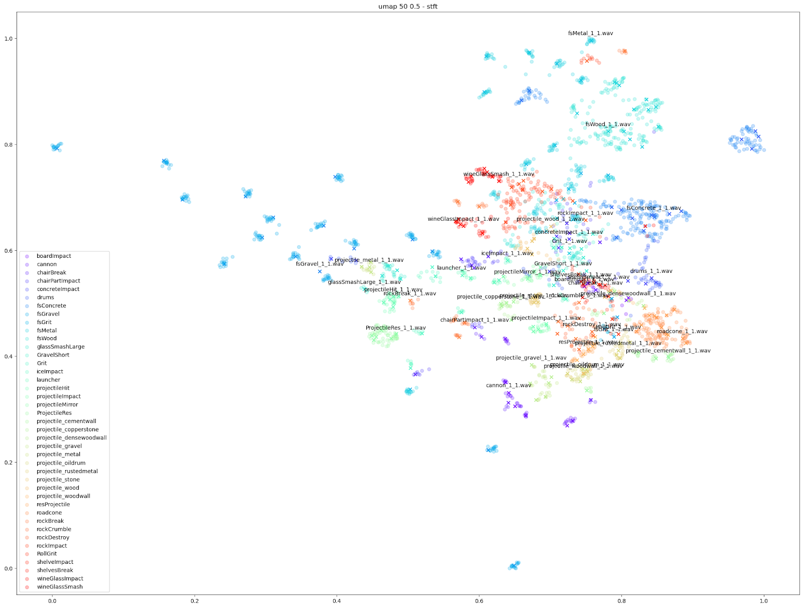 |
 |
.png) |
 |
Right click image "Open in new tab" for larger view.
As shown above, we found the UMAP and t-SNE algorithms working on STFT and MFCC++ (delta and delta-delta) provided the most useful plots.
References:
[1] - Hantrakul, L. “H. (2017, December 31). klustr: a tool for dimensionality reduction and visualization of large audio datasets. Medium. https://medium.com/@hanoi7/klustr-a-tool-for-dimensionality-reduction-and-visualization-of-large-audio-datasets-c3e958c0856c
[2] - Audio t-SNE. https://ml4a.github.io/guides/AudioTSNEViewer/
[3] -Bäckström, T. (2019, April 16). Deltas and Delta-deltas. Aalto University Wiki. https://wiki.aalto.fi/display/ITSP/Deltas+and+Delta-deltas

Comments